Lab 2: Problem Solving

Why are we here?

In Lab 1, you installed and configured the computing tools that we’ll use throughout this course, and for most classes in the SDS program. In this lab, we will begin learning the fundamentals of how to write programs in the language.

Whenever you’re programming a computer, chances are your program won’t work perfectly on the first try. That’s why we’ll also be developing one of the most important skill sets for a programmer to have: problem solving skills! Knowing basic trouble-shooting techniques you can apply when things don’t go according to plan is just as important as the plan itself.

Lab Goals

The purpose of this lab is to introduce you to working with R, and with resources and techniques for problem solving while using R.

After completing this lab, you should understand

• The RStudio interface
• How to use as a calculator
• How to store the results of your calculations as objects in the environment
• How to interpret error messages from
• How to find the built-in help resources in
• Identify working directories and navigate file paths

Optional Reading

Chapter 2: R basics and workflows Is a good additional reference for the material covered in this lab.

A note on labs

Each lab has the same structure:

• A Why are we here? section that explains how this lab relates to the previous labs, what motivates us to study and master the skills covered in this lab, and the specific learning goals for the lab activity.
  
• A lab instructions section, which includes explanations, examples and exercises that you need to complete
• A next steps section which explains what you need to do to finish this week’s lab and what you need to do to prepare for the next lab

To help you complete the exercises, most labs have an accompanying template file. You should download the template file at the start of each lab, move it into your SDS 100 project, and open the template in RStudio. This will help you answer the questions more efficiently you work through each lab.

Lab instructions

Setting up

1. Download the Lab 2 template.

2. Before you open the template, use your computer’s file explorer to move the template file you just downloaded out of your Downloads folder and into your SDS 100 folder.

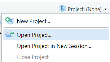
3. Then, open RStudio, and make sure you’re working in the SDS 100 project. If the Project pane in the top right of your RStudio window doesn’t show “SDS 100”, go to Open Project as shown below and navigate to your project.

   

4. Finally, open the template file in RStudio. The easiest way to do this is to go to the Files pane in RStudio, find the lab_02_problem_solving.qmd file from the list, and click on it.

   

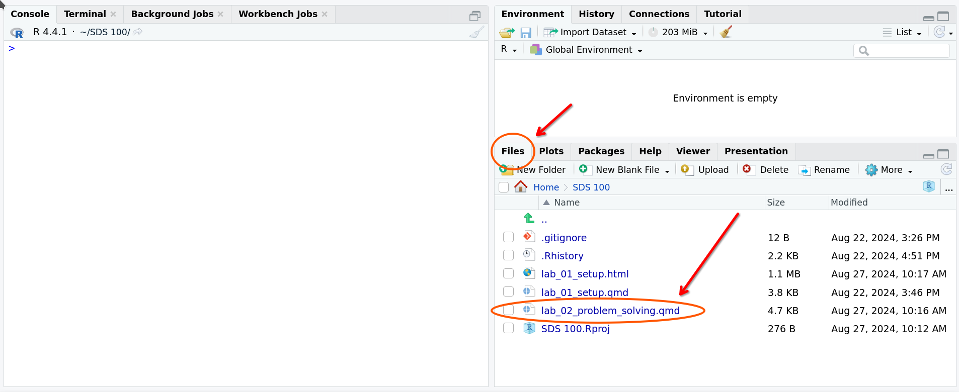
   If you don’t see a file named lab_02_problem_solving.qmd in the list, make sure you did steps 2 and 3 correctly. If you’ve double-checked your steps, and still don’t see it, ask your instructor for help.

R as a calculator

The first thing you can try to do with R is a familiar one - simply use it like a calculator. It is easy to forget because of all the other things it can do, but R at the lowest level is still just working with numbers.

Question

In the Console, enter 5 + 2 and press Enter to run the code.

Storing information in objects

Right now, the outputs of our code (in this case, the number 7) are just being shown to us. That can be helpful, but isn’t really the point of a programming language. We want to be able to save our results and build on them as we go. We can do that by assigning the output of the code we run into an object.

You can think of objects as boxes that store things. To create an object, we have to ask R to take the results of some code and assign those results to an object. We do this using the assignment arrow, <-. Let’s try it out.

Question

In the Console, type in result <- 5 + 2 and press Enter to run the code.

Then, type in applesauce <- 10 * 3 and press Enter to run the code.

You can see all of the objects you currently have in the upper right pane labeled Environment. At this point, you should see two objects in your environment: an object named result (which as the value 7) and and object named applesauce (which has the value 30). Objects can be named anything, as long as they 1) don’t start with a number, and 2) don’t contain any spaces.

Note that when you created result and applesauce, R didn’t print the results of 5 + 2 or 10 * 3 in the console. This is because creating an object is separate from showing it. Showing results is often called printing. In order to print an object, you can just write the name of it. When you run that, R will show you the object.

Question

Type result into the Console and press Enter to print it. Do the same with applesauce.

Objects are useful to use because we can use their names to represent their values in our code. For example, we can now add result and applesauce together, because result represents the value 7 and applesauce represents the value 30. Try it for yourself:

Question

In the Console, enter result + applesauce and press Enter to run the code.

We can even change what is stored inside those objects, then run the same code to get different results!

Question

In the Console, enter result <- 300 and press Enter to run the code. Then, try result + applesauce again. What has changed? Why?

Important

R will never save information in your environment unless you use the <- operator to store it. Printing information in the console is not the same as storing information for later!

R Functions and Arguments

Functions in R are like imperative sentences (e.g. “go”,“stay”, or “sleep”). They indicate to R that it should take some form of action. Telling R to use a function is described as “calling” a function. To call a function, its name must be followed by an opening and closing parentheses. For example, the Sys.Date function, followed by an opening and closing parenthesis, tells R to output the current date.

Sys.Date()

[1] "2024-12-19"

Now imagine we approached someone with an imperative sentence like “Close” or “Bring”. Their next question would likely be “Close what?” or “Bring what?”. In response, we might clarify what exactly they should be closing or bringing, e.g., “Close the door” or “Bring dessert”.

We face a similar need to be specific when calling functions in . The majority of functions we call need specific inputs in order for the instructions to make sense to . These inputs that specify the “what” or the “how” to a function are called arguments. Arguments to a function are always placed inside of the parentheses that follow a function.

Question

The sum() function adds up all of its arguments, and outputs the grand total. In the Console, enter sum(5, 2) and pressing Enter. What were the arguments you passed to the sum() function?

R Editor Panel

Up to this point, we have been writing R code in the Console pane. You’ll notice that when you direct your attention to the console, it will look like this:

>

When we execute code in the console, we get a result immediately. The console is a great space to work when we need to run a piece of code only once. However, the console is not a great space to edit code or to save code that we’ve written. This is why most of the code that you will write in this course and other SDS courses will be composed in the editor pane (which is typically located directly above the console). You’ll notice that when you direct your attention to the editor, the lab template for this lab will be open. In the open file, you will see text after a series of line numbers that look like this:

1
2
3

This is a file where you can compose, edit, and save code. In this file, you can also write text that explains the rationale for the code you’ve written, interprets the results, or offers additional contextual information regarding the data analysis.

Code Chunks

RStudio needs a way to know when we are switching from writing text about our code to actually writing code that we wish to execute. This is where code chunks come in to play. A code chunk is a space in a .qmd file where we can write code that we wish to execute. There are a few ways to create code chunks in RStudio:

First, we can place our cursors on a new line in the editor pane and type in the characters ```{r} to indicate the start of a code chunk. We can press the Enter key a few times to add some space for our code to go, and then type in the characters ``` to indicate the end of a code chunk. You’ll notice that when you do this, it creates a grey box with a green triangle icon in the upper right hand corner. The box will look something like this:

There’s another, simpler way to create a code chunk. Direct your attention to the upper right hand corner of your editor pane. You’ll notice a green icon with a plus sign (+) and the letter ‘C’, like this

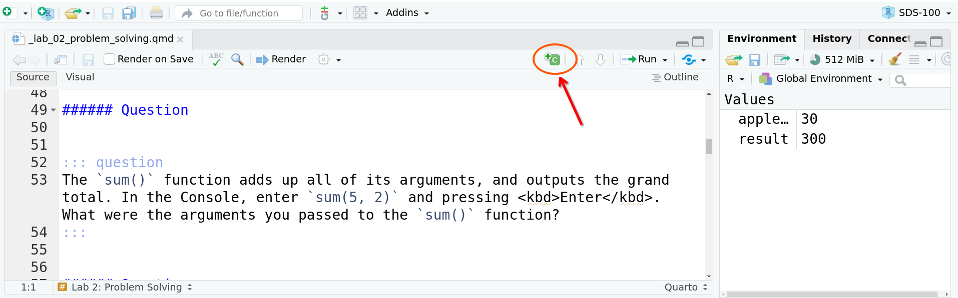
If you place your cursor on a new line and click that button, a code chunk will be automatically created on that line in the file. You’ll notice that the code chunk starts with ```{r} and ends with ```.

In this course, almost all of the code that we compose will be written in code chunks within .qmd files.

Question

In your template file, locate the code chunk that looks like this

```{r}
#| label: result_plus_applesauce
#| document: show

result <- 5 + 2
applesauce <- 10 * 3
```

Add result + applesauce to the blank line at the end of the code chunk. Click the green triangle “play” button in the upper right hand corner of the code chunk to execute the code in the chunk.

Just like when you ran this same code in the Console, here you’ve saved the result of 5 + 2 and the result of 10 * 3 to objects in your environment. You’ve also evaluated the result of adding the values stored in these two objects.

However, unlike when you ran this in the Console, this time around you have the ability to edit your code. For example, you could place your cursor on the line where you created the object for result, change the number 5 to 4, and then re-run the code to get a new result. You can also save this file so that you can re-run this code at a later date.

Warning

It’s very important that all ```{r} have a corresponding ```. If you don’t close a code chunk with ```, you will see that the code chunk extends to the end of your file. If you have an extra ``` in your file, you will notice that run buttons disappear in all of the code chunks below that extra ```.

If you ever notice that the green, triangular run buttons have disappeared from your code chunks, first make sure you are in the source editor mode, rather than visual. You can change this setting in the top bar of the editor pane. Next, look for an extra ``` in your .qmd file.

Commenting

Any text that you enter into a code chunk must be executable R code. For instance, check out what happens when we try to write some instructions in “plain English” at the bottom of our code:

result <- 5 + 2
applesauce <- 10 * 3
Place cursor here.

Error in parse(text = input): <text>:3:7: unexpected symbol
2: applesauce <- 10 * 3
3: Place cursor
         ^

We get an error because the words “Place cursor here” are not valid R code. If we want to add explanatory text to a code chunk, we need to preface that text with a hashtag (#) like this:

# This is a comment

This indicates that all of the characters following the hashtag should be ignored when it comes time to run the code.

Adding comments in code chunks is helpful for explaining what a piece of code is doing. This is important when sharing your code with others, or even reminding your future self why you took a certain approach. Check out how we use a comment to explain the code below:

# Below we create a vector of colors. To create a vector, we use the function c(), which is short for combine. 

colors <- c("red", "blue", "green")

Interpreting Error Messages

Often, something won’t go as planned. R has several ways to communicate with us, the most common of which are error messages. Error messages appear when something doesn’t work as anticipated. It is tempting to see them as denoting failure, but that is not the case. Error messages are a way for R to alert us to potential problems; they are R’s way of trying to communicate with us. The real danger comes where R does not tell us when something goes wrong.

First, it’s important to make some distinctions between the kinds of messages that R presents to us when attempting to run code:

Errors

Terminate a process that we are trying to run in R. They arise when it is not possible for R to continue evaluating a function. Like when we try to add letters together.

Warnings

Don’t terminate a process but are meant to warn us that there may be an issue with our code and its output. They arise when R recognizes potential problems with the code we’ve supplied.

Messages

Also don’t terminate a process and don’t necessarily indicate a problem but simply provide us with more potentially helpful information about the code we’ve supplied.

Check out the differences between an error and a warning in R by reviewing the output in the Console when you run the following code chunks.

Error in R

sum("3", "4")

Error in sum("3", "4"): invalid 'type' (character) of argument

Warning in R

vector1 <- c(1, 2, 3, 4, 5)
vector2 <- c(2, 4, 6, 8)
vector1 + vector2

Warning in vector1 + vector2: longer object length is not a multiple of shorter
object length

[1]  3  6  9 12  7

So what should you do when you get an error message? How should you interpret it? Luckily, there are some clues and standardized components of the message the indicate why R can’t execute the code. Consider the following error message that you received when running the code above:

Error in sum("3", "4") : invalid 'type' (character) of argument

There are three things we should pay attention to in this message:

1. The word “Error” indicates that this code did not run.
2. The text immediately after the word “in” tells us which specific function did not run.
3. The text after the colon gives us clues as why the code did not run.

Reviewing the error above, we can guess that there was a problem with the argument that we supplied to the sum() function, and specifically that we supplied an argument of the wrong type. This is because R interprets “3” and “4” as character stings (i.e., words) and not numbers, and it doesn’t know how to add words together.

Question

Edit the code below to correct the issues causing the “invalid ‘type’ (character) of argument” error, and then press the green “Play” button to run the corrected code.

sum("3", "4")

Preparing to Get Help

When we do get errors in our code and need to ask for help in interpreting them, it’s important to provide collaborators with the information they need to help us. Sometimes when teaching R we will hear things like: “My code doesn’t work!” or “I’m stuck and don’t know what to do,” and it can be challenging to suss out the root of the issue without more information.

Notice the left side of this document has a series of numbers listed vertically next to each line? These are known as line numbers. Oftentimes, if you are having an issue with your code and ask me to review it, we will say something like: “Check out line 53.” By this we mean that you should scroll the document to the 53rd line. You can similarly tell me or your peers which line of your code you are struggling with.

Referencing Resources

There are a number of resources available to help you recall how certain functions work.

Help pages

R help pages can be a great resources when you know the function you need to use, but can’t remember how to apply it or what its parameters are. Help pages typically include a description of the function, its arguments and their names, details about the function, the values it produces, a list of related functions, and examples of its use. You can access the help pages for a function by typing the name of the function with a question mark in front of it into our Console (e.g. ?log or ?sum).

Question

Imagine you recorded the temperature outside of your home at 11:00 am each day for ten day, and observed the following sequence of temperatures

68, 70, 78, 75, 69, 80, 66, 66, 79

First, insert a new code chunk into your Quarto document. Inside the code chunk, write code that will create a vector object named daily_temps to store these values.

Lastly, write code inside this code chunk that uses the sort() function to arrange these temperatures in descending order (i.e., from highest to lowest). Be sure to read the help page to find out how to change the sort order from ascending to descending!

When you think you’ve got it, run the code by pressing the green “play” button on your code chunk. You might not get it right the first time, and that’s OK! If you get an error message, reading your error message carefully, and practice your troubleshooting skills!

Cheatsheets

The R community has developed a series of cheatsheets that list the functions made available through some packages and their arguments. Cheatsheets are a great resources when you know what you need to do and what tools to use on a dataset in R, but can’t recall the function that enables you to do it.

Imagine that you needed to create a vector object representing the first 50 even numbers. You could do this by typing in the first 50 even numbers and combining them into a vector with the c() function, like this:

c(2, 4, 6, 8, 10, 12, 14, 16, 18, 20, 22, 24, 26, 28, 30, 32, 34,
  36, 38, 40, 42, 44, 46, 48, 50, 52, 54, 56, 58, 60, 62, 64, 66,
  68, 70, 72, 74, 76, 78, 80, 82, 84, 86, 88, 90, 92, 94, 96, 98,
  100
  )

But, this would be quite tedious and error prone. A better approach would be using an R function to generate such a sequence automatically.

Question

Use this cheatsheet to find an which R function will allow you to a generate a complex sequence of numbers. Then, use this function to generate a create a vector object named first_50_even representing the first 50 even numbers. Your code should print out this object after you create it, so you can double-check that it matches the sequence above.

Searching the Web

You can also search the web when you get errors in your code. Others have likely experienced that error before and gotten help from communities of data analysts and programmers. However, you should never copy and paste code directly from Stack Overflow. This violates the course policies on Academic Honesty. Instead you should use these resources to take notes and learn how to improve and revise code. Any time you reference Stack Overflow or any other Web resource to help you figure out an answer to a problem, you should cite that resource in your code. Here is how you would cite that a post from Stack Overflow in APA format:

Username of asker. (Year, Month Date). Title of page. Stack Overflow. Webpage URL

Question

Using a comment, add a properly formatted citation for this Stack Overflow post to the code chunk above.

File Paths and Organization

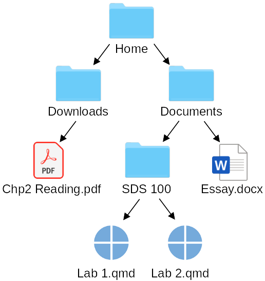
Computers allow you to save files, like Word documents or PDFs, so that you can access them whenever you need to. But, your computer doesn’t force all your files to be saved together in one place; your computer’s storage is divided into folders. For example, your computer comes with a folder named Downloads (where files downloaded from the internet are saved by default), and a folder named Documents (where new Word documents are saved by default).

Files that are saved on computer are called local files, while files that are elsewhere are called remote. Files that are in folders for syncing services like Dropbox, Google Drive, or similar services exist in an in-between, in that they are viable on your computer, but are downloaded on-demand whenever you try to open them. This can cause problems for R, so it is suggested you keep your code folders in non-synced locations.

The folders in your computer’s storage are arranged in a hierarchy, with one folder at the “top” of the hierarchy and others nested below them. Folders at lower levels of the the hierarchy are stored within the folders at higher levels. For example, your Downloads and Documents folders are actually nested within your user’s home folder (which is a folder you may not commonly encounter when browsing around your computer).

Folders and files in a heirarchy on your computer

Storage and items in a heirarchy in kitchen

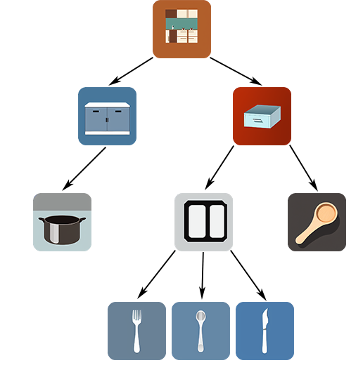
A good way to think about how your computer’s hierarchy of folders (usually called a file system) is organized is like a kitchen. You have access to everything, but you don’t want all your forks, spoons, plates, etc. all in one big pile on the floor. You organize them so they are easy to find and store. You may start with broad categories–you have a drawer for all your utensils–but inside that drawer it is broken down into smaller spaces; a spot for forks, spoons, knives, etc. The same principle is true of files. You create ever more specific spaces for things so they are easy to find later.

Making effective use of your file system

Unlike a kitchen, you can create new spaces for files whenever you want in the form of folders. For example, on the first day of class you made a special folder called an R Project, which we’ll learn more about in a minute. The power to create new folders is a useful organizational tool; it allows you to keep related files grouped together, but isolated from other irrelevant files.

It may be tempting to just store all your files in one place, like your Downloads folder or your Desktop. After all, it’s fewer clicks (or perhaps 0 clicks!) when you’re saving your work, and you can quickly accessing those folders. But, with all your files from all your classes in one place, you can’t quickly find what you need, just like if all your kitchen ware were in one giant pile. Also, if everything is in one place you can’t easily name your files, since all the names have to be unique (or you end up with several similar names like “Essay.docx”, “Essay (1).docx”, Essay (2).docx”, etc.). This makes searching for your files with the search bar tricky.

Furthermore, other programs on your computer might access and change files in this location (e.g., your web browser might clear your Downloads folder if you ask it to clean up space). For reasons like this, it’s a good idea to make folders on your computer to store work for different tasks. For example, it’s probably a good idea to make a folder for each of your classes inside your Documents folder. And it’s probably a good idea to make a folder just for homework assignments inside each of your class folders. Something like this:

Home
├── Documents/
│   └── Classes/
│       ├── SDS 100/
│       │   └── Homework
│       ├── SDS 192
│       ├── SDS 210
│       └── SDS 270
├── Downloads/
│   └── Memes
├── Pictures/
│   ├── Vacation
│   └── School
└── Music

R Projects & The working directory

Keeping track of where you save and store files on your computer is important to statisticians and data scientists who write code beyond just good organization: you need to tell R where files are so it can work with them. Without knowing exactly where these files are and what their exact names are, you won’t be able to access them. Often, the easiest way to make sure you can access files from within R is to make sure R’s working directory is the same folder as your files are in. The easiest way to do this is by making sure that you are in an RStudio Project, like the one from Lab 1.

While it’s not obvious, R is assigned a “working directory”: a folder on your computer where it is looking for files. Opening an RStudio Project sets R’s working directory to the Project directory. You can check and see what working directory R is currently watching by going into the Console, and using the command getwd(), which stands for “get working directory,” in the console.

getwd()

[1] "/home/will/Documents/Classes/SDS 100"

The getwd() function prints out the path to your current working directory. Mine will be different than your because we are on different computers! Think of paths as addresses that give directions to get to a specific folder on your computer. For example, the result from getwd() shown above says to get to the folder where the R program is currently watching on my computer, you have to:

1. Start the very top of the folder hierarchy
2. Then go to the folder name home
3. Then go to the folder named will
4. Then go to the folder named Documents
5. Then go to the folder named Classes
6. Then go to the folder named SDS 100

Since this particular path begins at the very top of the folder hierarchy (you can tell by the / at the very start), it’s called an absolute path. If you paste this command into your R console, we expect the path to your current working directory will be different, since your computer isn’t an exact copy of ours!

Question

Use getwd() to report the path to R’s current working directory

Why does the working directory matter?

For R to work on any files, it needs to know where they are. R Projects help R do that, because it will start looking for files inside the project folder, rather than way up at your Home folder. Let’s work through an example to see how this helps.

Go to the File menu in the upper left corner of your screen, and click on New File > Text File. This will open a new text file in R Studio. Inside this text file, Copy the sentence: “R is helpful, but needs very specific directions.” Save this file inside your SDS 100 project folder by going to the File menu in the upper left again, and clicking Save As ..., call it paths.txt. If you have your SDS 100 project open, you should be able to see your new file in the files pane in the lower right of R Studio. The video below shows an example of creating this file:

Say we wanted R to read this file for us, we have two options: give R the absolute path starting at our home directory, or the relative path, starting from our working directory. Where the absolute path to this file might look like:

"/home/will/Documents/Classes/SDS 100/paths.txt"

The relative path could cut out everything before the project folder, meaning all we would need for R to find the file is:

"paths.txt"

Let’s try it together.

Question

1. Insert a new code chunk into your Quarto document, and copy the code template below into your new code chunk

   # Replace the blank inside the parenthesis with the full path to the paths.txt file
   readLines(_______________________)

2. In the console, use getwd() to print out the path to your working directory.

3. Copy the output from getwd(), including the quotation marks

4. Replace the blank inside the parenthesis of the readLines() function with the path you copied

5. Add /paths.txt to the end of the path, inside the quotation marks

6. Press the green triangle “play” button on your code chunk. If you’ve specified the path correctly, R should print out what you wrote in that text file!

If you get an error message that ends with “No such file or directory” or “cannot open the connection”, double check the location you saved the paths.txt file, and double check that you specified the path correctly.

Reading files from relative paths will be super important when you start working with other people on code projects. Your partner in a group project can’t load a file from "/home/will/Documents/Classes/SDS 100/" because they won’t have a “will” folder on their computer. However, if you use a relative path, and everybody has the same files in their project, everyone will be able to use the same code.

Question

Use the readLines() function to print out what you stored in the paths.txt file, but this time, use a relative path to the paths.txt file to locate it. Remember, relative paths mean “look for this file starting from your current location”.

Remember, to use a relative path you have to know

1. The folder where your file is stored, and the precise file name
2. R’s current working directory
3. How to travel from the current working directory to the folder where your file is stored

If your current working directory is same folder where your file is stored, you can omit the names of any folders, and just put in the name of the file, like this: readLines("paths.txt")

Next Steps

Step 1: Compare solutions

Double check that you’ve completed each exercise in this lab, and have written a solution in your Quarto document. If so, render your Quarto document into an HTML file. Then, check your work for each exercise by comparing your solutions against our example solutions. The styling in the solutions file may look a bit different than yours, but the output should be the same.

Step 2: Complete the Moodle Quiz

Complete the Moodle quiz for this lab.

Step 3: Optional reading

To prepare for next week’s lab on data visualization, we encourage reading sections 4.1–4.4 in Data Science: A first introduction

References