Lab 7: Importing Data

Why are we here?

Nearly every lab in this course has used data, but all of that data has come from R packages. The reality is that most data is not part of an R package.

Data, like books or music, can have a variety of restrictions and protections. There is a wealth of “open-access” data, which is data that is shared publicly, often directly on the internet. In this lab, we will look at how to import this kind of publicly available data.

Lab Goals

The purpose of this lab is to teach you how to import data beyond just R packages.

After completing this lab, you should be able to import data stored as CSV files on the internet and from your local machine, and import data stored on the internet in Google Sheets.

You will know that you are done when you have created a rendered HTML document where the results match the example solutions.

Optional reading

The following are good additional resources for the material covered in this lab:

Sections 2.1 and 2.4 in Data Science: A First Introduction
Sections 8.1-8.2 in R for Data Science

In addition, the googlesheets4 README and the Getting Started vignette have many more examples of how you can work with data stored in Google Sheets.

Lab instructions

Setting up

First, download the First, download the Lab 7 template.
Before you open the template, use your computer’s file explorer to move the template file you just downloaded out of your Downloads folder and into your SDS 100 folder.
Then, open RStudio, and make sure you’re working in the SDS 100 project. If the Project pane in the top right of your RStudio window doesn’t show “SDS 100”, go to Open Project as shown below and navigate to your project.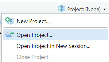
Finally, open the template file in RStudio. The easiest way to do this is to go to the Files pane in RStudio, find the lab_07_importing.qmd file from the list, and click on it.

If you don’t see a file named lab_07_importing.qmd in the list, make sure you did steps 2 and 3 correctly. If you’ve double-checked your steps, and still don’t see it, ask your instructor for help.

For today’s lab, we’ll need two new packages: googlesheets4 and janitor. Please install these packages now.

In addition to the googlesheets4 and janitor packages, we’ll also make use of the tidyverse package.

Question

Use the library() function to load the tidyverse, janitor, and googlesheets4 packages.

Importing Data from CSV files

Data files come in many shapes and sizes, but one of the most common is the CSV format. CSV is an acronym standing for comma-separated values. In this format, each row of the data is represented on a separate line of a text file, and the values that belong to each column (i.e., variable) are separated by commas.

In this section, we’ll learn how to load CSV files from the internet into

Coffee Ratings Data

The Coffee Quality Institute (CQI) is a non-profit organization that offers courses on coffee production, trains coffee raters, and offers quality certification services to coffee growers. Their website maintains a database of coffees that have been rated by the CQI’s reviewers.

In 2018, James LeDoux published a copy of the CQI’s database to enable other statisticians and data scientists to explore the factors that lead to highly rated coffee. Our goal will be importing James’ copy of the Robusta coffee bean ratings into R.

The link above takes you to a GitHub repository¹ which contains several different files and folders. In GitHub repositories, the README.md file often gives an overview of what is contained throughout the whole repository. This is often where you will find important documentation about the data set.

Question

Spend a minute reviewing the README file in the coffee quality rating GitHub repository. Which of the following is not an aspect the coffees were rated on?

Body
Cup Cleanliness
Bitterness
Moisture

Locating the URL for a file in a GitHub repository

To import the data file we want (the Robusta coffee ratings), we’ll need to search through the GitHub repository, and locate a link to that specific CSV file.

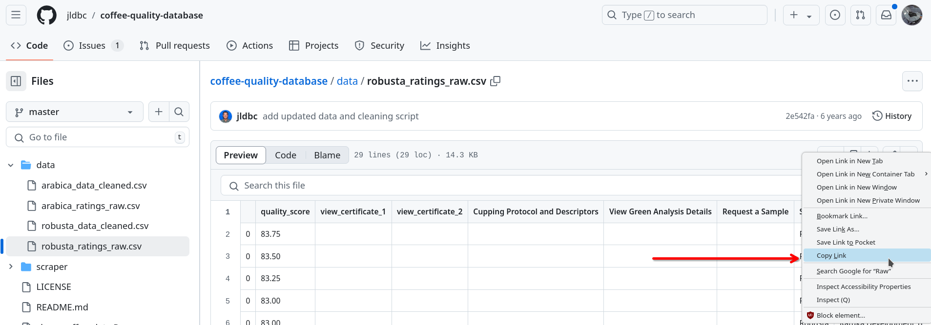
From the repository’s home page, click on the folder named data. Once inside the data folder, click on the file named robusta_ratings_raw.csv. This should take you to a page where data is displayed in a table. This is a user-friendly display, but it’s not quite the page we’re looking for.

To find a link to the actual CSV file, look for a button labelled “Raw” towards the top-right corner of the table.

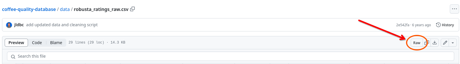
Right-click (or two-finger click if you’re on a Mac) on this “Raw” button, and click on the option in the menu that says something like “Copy link” (the exact phrase differs from browser to browser).

Congratulations, you’ve found the URL (i.e., link) that links to the Robusta coffee ratings file!

Importing data using `read_csv()`

So far, we have identified the URL where the data are stored, but we still need to import these data into . To import CSV files, we’ll use the read_csv() function from the readr package, which is part of the tidyverse. By loading the tidyverse, we have automatically loaded the readr package.

The read_csv() function works by taking in a file path describing the location of the file as it’s first argument, and returning a data frame holding those data. Importantly, a URL is one type of file location the read_csv() function understands. This means we can take the URL for the “raw” Robusta coffee ratings, and place it directly inside the parenthesis of the read_csv() function to import these data!

Question

Insert a new code chunk in your Quarto document, and copy the code template below into this code chunk.

____________  read_csv(__________)
print(robusta_raw)

Then, copy the “raw” URL for the robusta_ratings_raw.csv from GitHub, and paste this URL inside the call to read_csv(). Don’t forget to put quotation marks around the URL!

Use the <- assignment operator to store the output from the read_csv() function in an object named robusta_raw.

Finally, confirm that the data was imported correctly by printing the robusta_raw object.

Question

Use glimpse() to get a quick overview of the robusta_raw data. Then, use the output from glimpse() to answer the following questions.

How many variables are measured in these data?
How many variables have names with ... in them?
How many variables have names with spaces in them?

Cleaning up Variable names

Just like authors of academic articles might use APA or MLA style when writing papers, programmers follow style guidelines when they write their code. Following a common set of conventions helps to make code easier to read and understand. One convention for R programmers is to consistently use lower case letters, and not use spaces, when naming variables.

Unfortunately, the robusta_raw data set does not follow this convention. We could manually update these variable names using dplyr::rename(), but this would be tedious with dozens of variable names to edit. Instead we’ll get acquainted with a new tool that will help us be more productive by renaming all the columns to follow R’s naming conventions: the clean_names() function from the janitor package!

Question

Insert a new code chunk in your Quarto document, and copy the code template below into this code chunk.

___________ <- clean_names(__________)
glimpse(robusta_cleaned)

Fill in the blank inside the clean_names() function with the robusta_raw data frame object. Then, use the <- assignment operator to store the output from the clean_names() function in a new data frame object named robusta_cleaned.

Finally, run the glimpse() function to inspect the newly created robusta_cleaned data frame. How have the variable names changed after using the clean_names() function?

More Practice: Assemble the Avengers

Question

Investigate the online repository for the avengers data from FiveThirtyEight, which is all about Marvel comic book characters.

Then, import the avengers.csv file, and then clean up the variable names. Finally, use the glimpse function to answer the following question: how many variable’s in this data set contain numeric data?

Importing Data from Google Sheets

So far in this lab, we’ve imported data that exist publicly as CSV files. But CSV files are just one of many ways data are stored and distributed. Another common place to store and share data is on Google Sheets. In this next section, we will learn how to access data stored in a Google Sheet directly from R by using the googlesheets4 package.

Setting up `googlesheets4`

While files on Google Sheets can be made public, the vast majority of files are kept private and are only accessible to people with authorized Google accounts. The googlesheets4 package makes it easy to access private files (provided you have an authorized Google account!) by coordinating the process of logging into your Google account from within R.

This section will walk you through how to give googlesheets4 permission to access Google Sheets through your Google account. If done properly, you will only need to follow these steps once per computer.

Read Carefully!

Attention to detail is needed when setting up the googlesheets4 package. Please read though these instructions fully before you start the installation, so you can anticipate what you’ll need to do in each step.

Step 1: Request Access from R

Begin the process by running the command gs4_auth() in the console. After running this command, one of two things may happen:

Your web browser will open a new tab
will ask you a question in the console
```
The googlesheets4 package is requesting access to your Google account.
Enter '1' to start a new auth process or select a pre-authorized account.
```
If you see this question, enter the number 1 in the console, and press Enter. This should cause your web browser to open a new tab.

may also ask you the following questions in the console:

Is it OK to cache OAuth access credentials in the folder
~/Library/Caches/gargle between R sessions?

The httpuv package enables a nicer Google auth experience, in many cases.
It doesn't seem to be installed.
Would you like to install it now?

It is recommended that you select option 1 for both of these questions (Yes, allow caching, and Yes, install the httpuv package).

Step 2: Allow Access from your Web Broswer

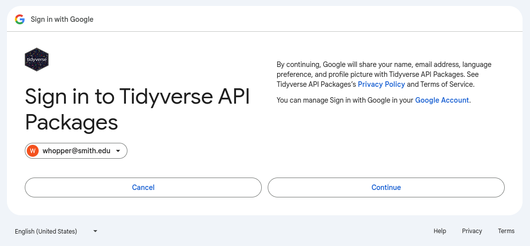
Once R opens your web browser, you may first see a page asking you choose which Google account you would like to grant access. You should choose to authenticate with your Smith account:

Next, you will be asked to accepted the terms of service for the “Tidyverse API” packages. Press continue.

After pressing Continue, you will arrive on a page with three check boxes. Two are checked off by default, but you need to check the third one before continuing!

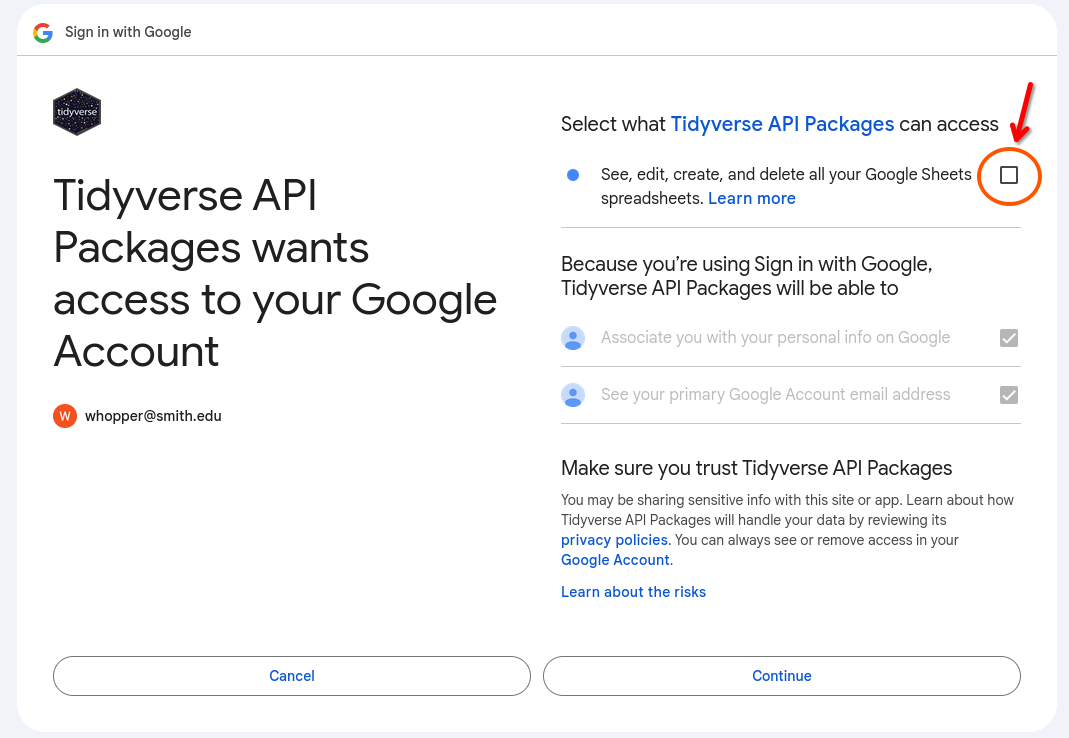
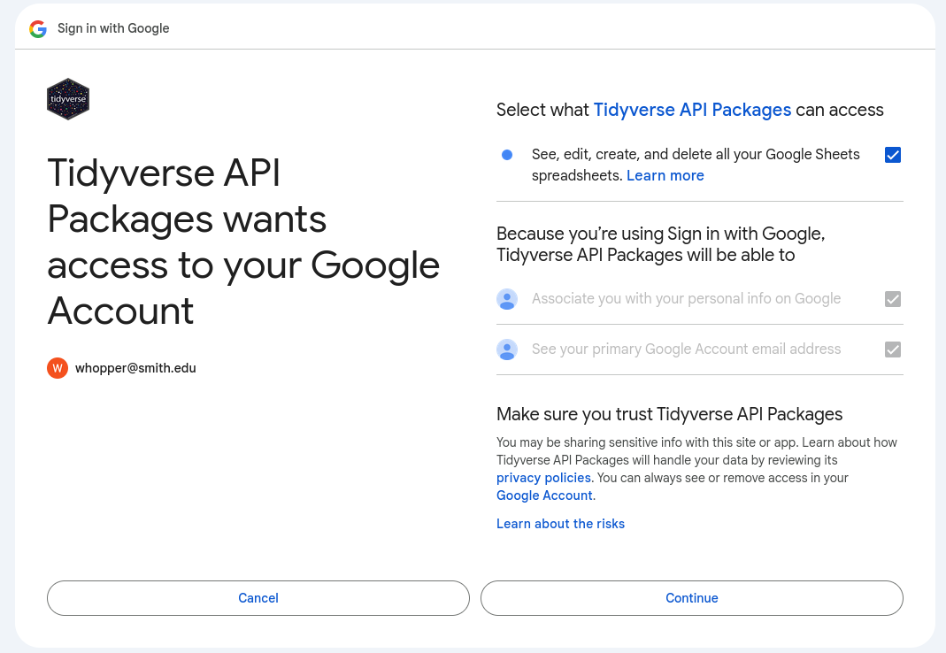
Check the third box (as shown in Figure 2 above) and then click Continue.

Finally, you should next be taken to a blank webpage that has the following text in the top left hand corner:

Authentication complete. Please close this page and return to R.

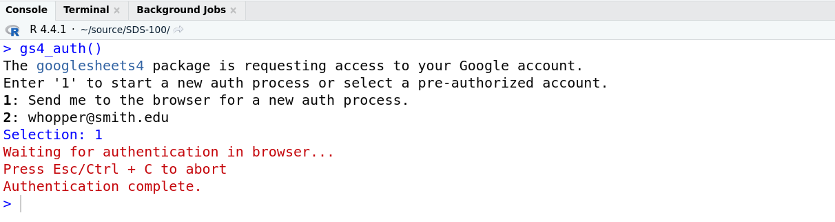
If you see this page, you can close this tab and return to RStudio. Back in RStudio you should see a message saying “Authentication Complete”, similar to this:

Congratulations, you have successfully configured the googlesheets4 package! You’re now ready to start using it to import data.

Mind the Gap

In this section, we’ll use data from the Gapminder foundation, an educational non-profit that takes a data-driven approach to fighting misconeptions and ignorance about social issues worldwide. For example, their Dollar Street project contextualizes income data from individual families around the world with photographs and videos.

Today, we’ll be working with a data set published by Gapminder that describes life expectancy, population, and Gross Domestic Product per capita over time for each country in the world. This data is published here, as a Google Sheet. For this lab, we’ll just be working with the data from the first tab, which describes countries located in Africa.

Importing data using `read_sheet()`

The read_sheet() function works similarly to the read_csv() function. It takes in information describing the location of the data as it’s first argument, and returns a data frame holding those data. But the read_sheet() only understands a single type of URL: A URL describing the location of a Google Sheet.

Question

Insert a new code chunk into your Quarto document, and copy the code template below into this chunk.

_________ <- read_sheet()
print(gapminder)

Then, navigate to the Gapminder Google Sheet, and copy the URL from the address bar. Paste this the URL inside the call to the read_sheet() function, with quotation marks around the URL. Next, use the assignment operator to store the output from the read_sheet() function in an object named gapminder. Finally, confirm that the data was imported correctly by printing the gapminder object.

Question

Above, we discussed the difference between read_sheet() and read_csv(). Copy your code from the previous answer into a new code chunk below. Then, replace read_sheet() with read_csv(), and run the code again (this command may take a several moments to finish running).

What happens when you use read_csv() instead of read_sheet() on a Google Sheet URL? Hint: Consider the number of rows and columns. Is this what you expect?

Reading data from your local machine

Now that we have learned a couple of methods for reading data from the web, let’s apply what we learned about file paths in Lab 2 to read in data files stored on our own computer. We’ll learn how to do this by working with a data set of product reviews collected from JD.com, an e-commerce website similar to Amazon.com that is popular in China.

First, download the dataset to your computer. Clicking this link will download a file name 89p4bsmdpd-1.zip file into your computer’s Downloads folder. This file isn’t our data; rather, the data we want is stored inside a special type of compress folder called a “zip file”. We need to extract the data from this zip file before we can use it.

Question

Extract the data file named product review text.csv from the zip file you downloaded, and move it into your SDS 100 project folder.

If you’ve never extracted files from a zip file before, here are some instructions you might find helpful:

Because the file ends the .csv extension, let’s try importing the file with the read_csv() function, and storing the data in an object named JD_product_reviews. Note that in code below, our path to the product review text.csv file assumes the data file is in the same folder as the Quarto document.

JD_product_reviews <- read_csv("product review text.csv")

Error in nchar(x, "width"): invalid multibyte string, element 1

But instead of data, we get a strange error message. This message tells us that our data is likely stored using a special type of character encoding. In this case, the data are stored in a character encoding specialized for Chinese languages.

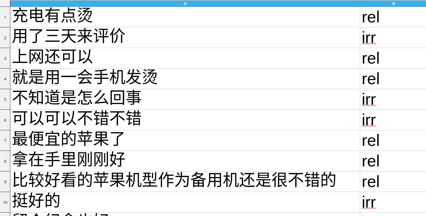
When a data set uses a specialized character encoding, figuring out what the proper encoding to use might be difficult. A great first step is to use the guess_encoding() function from the readr package. Let’s see what encoding is detected in the product review text.csv file:

guess_encoding("product review text.csv")

# A tibble: 4 × 2
  encoding confidence
  <chr>         <dbl>
1 GB18030        1   
2 EUC-KR         0.78
3 Big5           0.7 
4 EUC-JP         0.56

The file contents is similar to several encoding, but is most similar to GB18030 encoding. Let’s try importing the product review text.csv file again, but this time, we’ll tell to use the GB18030 encoding when reading the file.

Question

Use the locale() function (which comes from the readr package) to create an object representing a Chinese locale that uses the GB18030 encoding, just like the example below:

chinese_locale <- locale(encoding = "GB18030")

Then, try using the read_csv() function to import the product review text.csv file and store the data in an object named JD_product_reviews again. But this time, pass the locale object you created into the read_csv() function using the locale argument.

Check that the data were imported properly by printing out the JD_product_reviews object; the data should look like the screenshot above.

Always check the file extension!

When working with a data file, the first thing you should check is what format the file is in. The format is usually denoted by the three letters following the final period in the file’s name These letters are known as the file extension. For example, the letters csv following the last period in the product review text.csv indicate that it is a CSV file.

Unfortunately, your operating system may hide file extensions when browsing files. To make matters worse, some programs on your computer (e.g., Microsoft Excel, or Numbers) can open many different types of files. So the icon you see next to file name may be the same for two completely different types of files!

You can usually get more information about the file extension by right-clicking (or pressing the Ctrl key and clicking) on a file, and choosing an option like “Get Info” or “Properties” from the menu.

Next Steps

Step 1: Compare solutions

Render your Quarto document, and trouble-shoot any errors that might appear. If you’ve done each exercise correctly, the output in your rendered HTML file should match the output in the Lab 7 solutions file.

Step 2: Complete the Moodle Quiz

Complete the Moodle quiz for this lab.

Footnotes

We won’t be learning how to use GitHub in SDS 100. However, GitHub is introduced in SDS 192 and is used extensively in upper-level SDS classes.↩︎

Why are we here?

Lab instructions

Setting up

Question

Importing Data from CSV files

Coffee Ratings Data

Question

Locating the URL for a file in a GitHub repository

Importing data using read_csv()

Question

Question

Cleaning up Variable names

Question

More Practice: Assemble the Avengers

Question

Importing Data from Google Sheets

Setting up googlesheets4

Step 1: Request Access from R

Step 2: Allow Access from your Web Broswer

Mind the Gap

Importing data using read_sheet()

Question

Question

Reading data from your local machine

Question

Question

Always check the file extension!

Next Steps

Step 1: Compare solutions

Step 2: Complete the Moodle Quiz

Footnotes

Importing data using `read_csv()`

Setting up `googlesheets4`

Importing data using `read_sheet()`