Code
acs_df <- openintro::acs12Often, when we find data for a project it is not quite ready for use yet. Maybe the data are too large and you only need some subset of the observations or variables. Alternatively, you may have a variable that needs to be changed. For example, you might want to change a variable from being numeric (income in dollars) to a categorical measure (high, medium, low income). The process of wrangling your data is a vital step that makes your data usable for visualization or analysis.
The purpose of this lab is to get an introduction to the logic of data “wrangling” (i.e., transforming the data to the format you need for visualization/analysis).
You will be learning how to use the select(), filter(), mutate(), and arrange() commands from the dplyr package to alter a data frame.1
After completing this lab, you should be able to transform a data frame by subsetting variables and observations, generating new variables, and sorting your data by values.
You will know that you are done when you have created a rendered HTML document where the results match the example solutions.
4.1-4.3 in R for Data Science is a good additional resource for material covered in this lab.
Download the Lab 4 template.
Before you open the template, use your computer’s file explorer to move the template file you just downloaded out of your Downloads folder and into your SDS 100 folder.
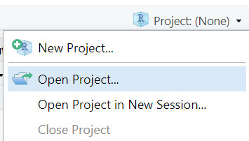
Then, open RStudio, and make sure you’re working in the SDS 100 project. If the Project pane in the top right of your RStudio window doesn’t show “SDS 100”, go to Open Project as shown below and navigate to your project.
Finally, open the template file in RStudio. The easiest way to do this is to go to the Files pane in RStudio, find the lab_04_wrangling.qmd file from the list, and click on it.
If you don’t see a file named lab_04_wrangling.qmd in the list, make sure you did steps 2 and 3 correctly. If you’ve double-checked your steps, and still don’t see it, ask your instructor for help.
![]()
We will be relying on the dplyr package found in the tidyverse for all our data wrangling. To complete this lab you will need to load the tidyverse package (refer back to Lab 3 for instructions on how to load packages).
To learn the fundamentals of data wrangling, we’ll work with a sample of data from the US Census Bureau’s American Community Survey (ACS). This sample of data, named acs12, is made available through the openintro package. So to complete this lab, you’ll also need to install and load the openintro package. Take a moment to install this package now, and refer back to Lab 1 for instructions on how to install packages if you need a refresher.
Once the openintro package is installed, we’ll need to import the acs12 data set and store a copy of it as an object in our environment. The code below shows you how to do this:
acs_df <- openintro::acs12The double colon operator (::) provides explicit access to objects within packages. So openintro::acs12 means “Reach into the openintro package, and retrieve the ac12 object from within”.
We’ve chosen to name this object acs_df. We could have named this object anything we wanted, but we chose the name acs_df because it helps us that is holds data from the ACS survey in a data frame object. When you choose a name for your objects, you should always try to choose a name that is both short and informative.
Insert a new code chunk in your Quarto document. In this code chunk, write code that will:
tidyverse packageacs12 data set from the openintro package, and store a copy of it as an object named acs_df in our environment.acs_df dataThe acs_df data contains measurements of several demographic and employment-related variables. Each observation represents an individual respondent, meaning that our units are individual people living in the United States.
The glimpse() function (which comes from the dplyr) package is a useful tool for getting a quick and compact overview of a data set’s contents. Let’s use this function now to learn a bit more about the data contained in the acs_df object.
glimpse(acs_df)Rows: 2,000
Columns: 13
$ income <int> 60000, 0, NA, 0, 0, 1700, NA, NA, NA, 45000, NA, 8600, 0,…
$ employment <fct> not in labor force, not in labor force, NA, not in labor …
$ hrs_work <int> 40, NA, NA, NA, NA, 40, NA, NA, NA, 84, NA, 23, NA, NA, N…
$ race <fct> white, white, white, white, white, other, white, other, a…
$ age <int> 68, 88, 12, 17, 77, 35, 11, 7, 6, 27, 8, 69, 69, 17, 10, …
$ gender <fct> female, male, female, male, female, female, male, male, m…
$ citizen <fct> yes, yes, yes, yes, yes, yes, yes, yes, yes, yes, yes, ye…
$ time_to_work <int> NA, NA, NA, NA, NA, 15, NA, NA, NA, 40, NA, 5, NA, NA, NA…
$ lang <fct> english, english, english, other, other, other, english, …
$ married <fct> no, no, no, no, no, yes, no, no, no, yes, no, no, yes, no…
$ edu <fct> college, hs or lower, hs or lower, hs or lower, hs or low…
$ disability <fct> no, yes, no, no, yes, yes, no, yes, no, no, no, no, yes, …
$ birth_qrtr <fct> jul thru sep, jan thru mar, oct thru dec, oct thru dec, j…The output reveals several key features:
<int> and <fct> labels following each variable name tell us how the measurements of that variable are encoded. The <int> label (short for “integer”) tells us the variable is represented with numbers. The <fct> label (short for “factor”) tells us the variable is represented using discrete categories.Based on the output from the glimpse() function, answer the following questions:
One crucial tool that simplifies data wrangling in is the pipe operator.
|>. You may occasionally see the older version of a pipe (%>%) online or in other classes, but both pipes work the same way.x |> f(y) means the same thing as f(x, y).acs_df data frame, and then only keep the variables income, age, and gender, and then only keep observations where the respondent is female.subset_df <- acs_df |>
select(income, age, gender, hrs_work, time_to_work) |>
filter(gender == "female")You may find the following video about the pipe operator helpful. Please note that while the video refers to the old pipe (%>%), the content also applies to the new pipe (|>).
The select() function allows us to choose which variables to subset from a data frame.
Datasets may contain dozens, or even hundreds of variables, but a researcher is often only interested in some of these variables. The extra variables or observations not only make it harder to sort through and identify the data you want, but can also slow down your computer as it reads through gigabytes of data. Before working with data, you should identify its codebook, which should have information about each of the variables and how they are measured. Codebooks are a major resource for you to identify what data you do and do not want.
To make the data easier to work with (and potentially save huge amounts of computer memory) we can use the select() command to only keep the variables we want to analyze. Figure 1 illustrates the logic of the select() function. The number of columns (representing variables) is reduced from five to three, as we only told R to select columns 2, 3, and 5.
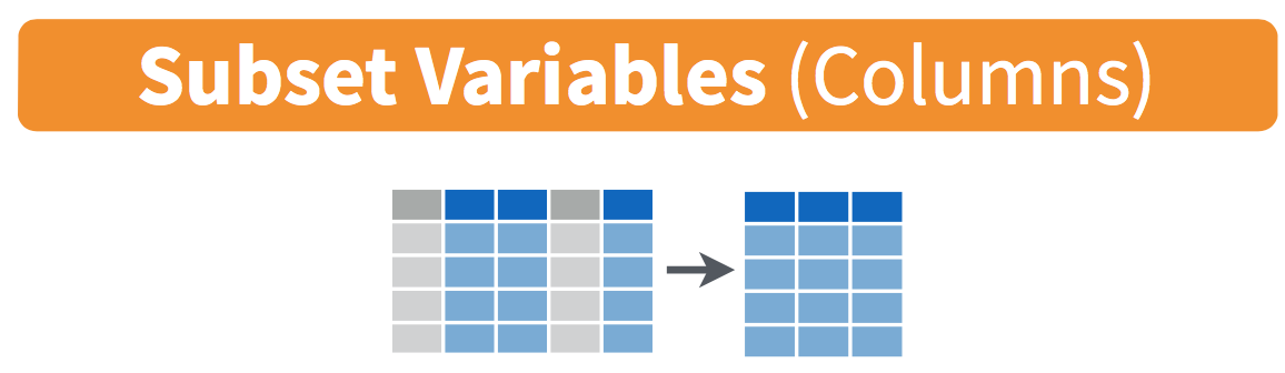
select() function. The variables in blue are selected, while the variables in grey are discarded.
The example code below takes the acs_df data frame, and then only keeps the variables income, employment and age.
acs_df |>
  select(income, employment, age)
# A tibble: 2,000 × 3
income employment age
<int> <fct> <int>
1 60000 not in labor force 68
2 0 not in labor force 88
3 NA <NA> 12
4 0 not in labor force 17
5 0 not in labor force 77
6 1700 employed 35
7 NA <NA> 11
8 NA <NA> 7
9 NA <NA> 6
10 45000 employed 27
# ℹ 1,990 more rowsHowever, if we print out the acs_df data set, the other 10 variables are still present.
acs_df# A tibble: 2,000 × 13
income employment hrs_work race age gender citizen time_to_work lang
* <int> <fct> <int> <fct> <int> <fct> <fct> <int> <fct>
1 60000 not in labor f… 40 white 68 female yes NA engl…
2 0 not in labor f… NA white 88 male yes NA engl…
3 NA <NA> NA white 12 female yes NA engl…
4 0 not in labor f… NA white 17 male yes NA other
5 0 not in labor f… NA white 77 female yes NA other
6 1700 employed 40 other 35 female yes 15 other
7 NA <NA> NA white 11 male yes NA engl…
8 NA <NA> NA other 7 male yes NA engl…
9 NA <NA> NA asian 6 male yes NA other
10 45000 employed 84 white 27 male yes 40 engl…
# ℹ 1,990 more rows
# ℹ 4 more variables: married <fct>, edu <fct>, disability <fct>,
# birth_qrtr <fct>The acs_df data set is unchanged because we did not assign the output from the select() function. Instead, we simply printed the output into the console.
If we wanted to save these changes permanently, we need to assign them to an object by using the assignment operator <-, and creating a new object name. For example:
acs_subset <- acs_df |>
  select(income, employment, age)
would store our three variables in a new object named acs_subset.
If we wanted to modify the acs_df data set, and remove the other 10 variables permanently, we would place the acs_df object on the left hand side of the assignment operator.
Insert a new code chunk into your Quarto document. Then, copy the template code below into this code chunk:
acs_df |>
  select(________)
Modify this template so that the select() function keeps only the variables married, race, and edu.
Insert a new code chunk into your Quarto document, and write code that will
employment, time_to_work, and hrs_work variables from the acs_df data set.acs_employment.acs_employment data.Another way we may want to wrangle our data is to evaluate a subset of the observations.
The filter() function allows us to subset our data by only keeping the observations that fit a condition. Perhaps we are interested in respondents who are over the age of 65, or only the non-white sample. The filter() function evaluates a logical expression based on a value of one or more columns, and only keeps those observations for which the expression is true.
Figure 2 illustrates the logic of the filter command.
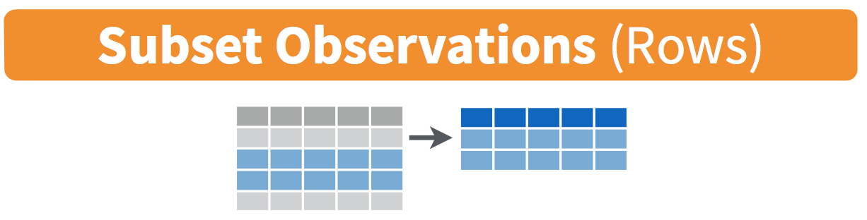
filter() function. Here, only the 2nd and 3rd rows (in blue) meet the condition and are kept. The 1st and 4th rows (in grey) do not meet the condition and are discarded.
The code below takes our saved data frame, and then only keeps rows where the observed gender is is female. The equality comparison operator == is how we tell “Find the rows where the gender variable equals the value "female"”.
Don’t confuse the == operator with the = sign. The == is a test for equality, whereas = is an assertion of equality. Thus, a == b will return TRUE or FALSE (depending on whether a actually equals b or not) whereas a = b will set the value of a to be equal to the value of b.
Run the code below, and note the number of rows in the output. Is it different than the original data frame?
acs_df |>
  filter(gender == "female")
What if our variable is numeric instead of categorical? We can use > or < to instruct R which cases to keep. For example, the code below only keeps observations where the age of the respondent age is 30 or less.
acs_df |>
  filter(age <= 30)
We can also filter by multiple conditions. For example, we may only be interested in female respondents under the age of 30. We use & (AND) to only keep cases that fit both conditions. So, someone who is under 30 and is female.
acs_df |>
  filter(age <= 30 & gender == "female")
Alternatively, we use | (OR) to say we want to keep observations that meet either of the conditions. So anyone who is under 30, or is female. Notice the tibble below contains a lot more cases.
acs_df |>
filter(age <= 30 | gender == "female")Insert a new code chunk into your Quarto document, and copy the template code below into your new code chunk.
acs_df |>
  filter( ______  & _______  )
Modify this template so that the filter() function only keeps observations where time_to_work is greater than or equal to 35 minutes and income is strictly greater than fifty thousand dollars ($50000).
mutate() is a powerful tool when wrangling data because it allows us to create new variables based on the values of other variables.
Figure 3 illustrates the logic of the mutate() function.
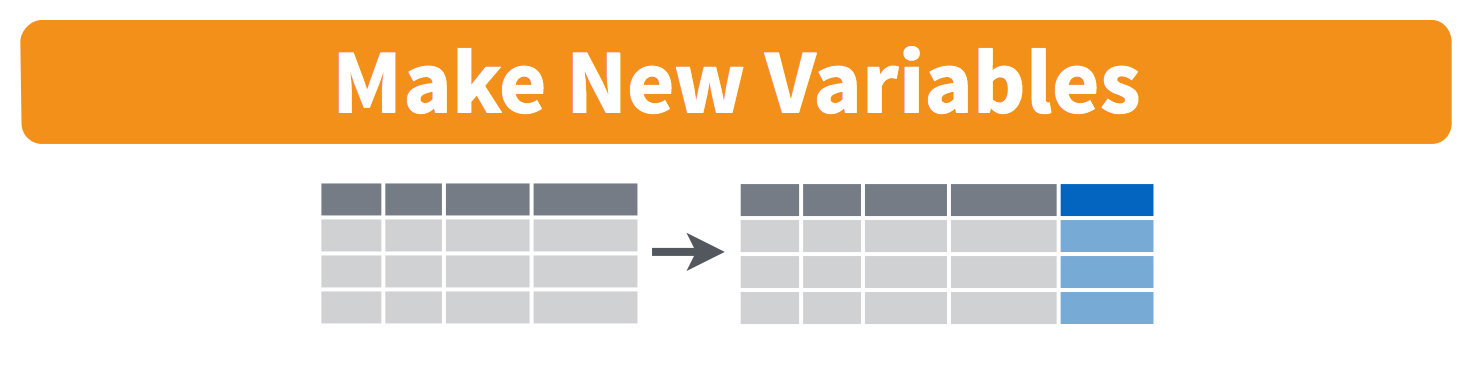
mutate() function. The existing variables (in grey) are unchanged, while a new variable (in blue) is created.
For example, in the ACS data set the variable income is measured in dollars, so the scale is quite large, ranging from a low of $0 to a high of $450,000. Given how large the numbers are, we may want to divide this value by 1,000 so we can get a new variable that measures income in $1,000 increments.
The example code below selects four variables from the acs_df data set (including income), and then uses the mutate() function to create a new column named income_1000 to hold our new “income in thousands of dollars” variable. This new variable is created by dividing the existing income variable by 1,000.
subset_df <- acs_df |>
  select(income, age, hrs_work, time_to_work) |>
  mutate(income_1000 = income / 1000)
subset_df
# A tibble: 2,000 × 5
income age hrs_work time_to_work income_1000
<int> <int> <int> <int> <dbl>
1 60000 68 40 NA 60
2 0 88 NA NA 0
3 NA 12 NA NA NA
4 0 17 NA NA 0
5 0 77 NA NA 0
6 1700 35 40 15 1.7
7 NA 11 NA NA NA
8 NA 7 NA NA NA
9 NA 6 NA NA NA
10 45000 27 84 40 45
# ℹ 1,990 more rowsNotice that the name of the new variable goes on the left hand side of the equals sign, and your instructions about how to compute this new variable go on the right hand side. Also notice that we are permanently changing the subset_df data set by using R’s assignment operator to overwrite the original data set with our updated data set that includes the income_1000 column.
Use the mutate() command to generate a new variable in the subset_df data frame that measures age in months instead of years.
Lastly, the arrange() function is a tool that orders the rows of a data frame by the values of a variable. For example, you could sort the data by income with the lowest income values being in the first rows, and the highest in later rows.
subset_df |>
  arrange(income_1000)
If you want to reverse the order, you can add desc() to the command.
 subset_df |>
arrange(desc(income_1000))Insert a new code chunk into your Quarto document, and copy the template code below into your new code chunk.
subset_df |>
  arrange(_________)
Modify this code template so that the arrange() function sorts the subset_df data frame by the hrs_work variable.
Insert a new code chunk into your Quarto document, and write code that will arrange the subset_df data frame by time_to_work in descending order.
Because of our pipe operator, rather than having separate commands that filter, select, mutate, or arrange our data, we can combine multiple instances of these tools into a single pipeline. For example, the code below keeps the variables age, gender, and race, and then only keeps observations with age greater than or equal to 75. Order does matter. For example, if we did not select the age variable, then we would not be able to filter the data by age (because we dropped it!).
acs_df |>
  select(age, gender, race) |>
filter(age >= 75)Insert a new code chunk into your Quarto document, and copy the template code below into your new code chunk.
acs_df |>
  select(____________) |>
  filter(____________)
Modify this template so that the select() function keeps just the variables hrs_work, income, and married, and the filter() function keeps just the observations where income is less than $ 30,000.
Insert a new code chunk into your Quarto document, and write a data wrangling “pipeline” that will
income_1000 that measures income in thousands of dollars (instead of dollars)Double check that you’ve completed each exercise in this lab, and have written a solution in your Quarto document. If so, render your Quarto document into an HTML file. Then, check your work for each exercise by comparing your solutions against out example solutions.
Complete the Moodle quiz for this lab.
During this week, you should begin Phase 1 of the final project. See the Final Project page for full instructions.
To prepare for next week’s lab on summarizing, we encourage reading section 4.4-4.5 in R for Data Science.
The pipe operator in R was inspired by the pipe operator from UNIX (|).↩︎