Lab 5: Summarizing Data

Preamble

The purpose of this lab is to practice computing summary statistics for categorical and numeric variables, including summaries of specific groups of observations within a larger data set. You will also practice recognizing which summary statistics are appropriate for specific types of data-based questions.

After completing this lab, you should be able to use R’s built-in summary functions, together with the group_by() and summarize() functions from the dplyr package, to compute a variety of summary statistics.

You will know that you are done when you have created a rendered file where the results match the examples in this HTML file.

Why are we here?

Data is a valuable resource, but raw data alone is not always useful to anyone. When was the last time scrolling through a large spreadsheet of information told you something particularly interesting about the world? Data sets usually need to be arranged in some way in order to gain insight from them.

In this class, we’ve already encountered one technique for identifying patterns in large data sets: data visualizations! In today’s lab, we’ll practice another technique for arranging data in order to make sense out of it: computing summary statistics.

When you compute a summary statistic, you are taking the values from many different individual observations of one variable, and “boiling them down” to one representative value. What kind of summary statistic you choose to compute depends on what type of variable you want to summarize, and what you want to learn about that variable.

In many cases, something as simple as comparing the average value of a single variable across different groups produces enough information to draw insight.

Lab instructions

Setting up

Download the Lab 5 template.

Warning

Before you begin:

• Move the template file you just downloaded from your Downloads folder into the SDS 100 folder that you created in Lab 1.

• Make sure that within RStudio, you’re working in the SDS 100 project that you created in Lab 1.

For more detailed instructions on either of the above, see Lab 2.

Optional reading

4.4-4.5 in R for Data Science is a good additional resource for the material covered in this lab.

Common Summary Statistics

A list of all the summary statistics in the world would go on for pages and pages. Table 1 below lists 7 summary statistics that are useful in a wide variety of contexts. In R, each of these summary statistics is computed by using a different R function on the variable you want to summarize.

Table 1: Seven commonly-used summary statistics

Statistic	Meaning	R Function
Total	The sum of all values in a numeric variable	sum()
Mean	The average value of numeric variable	mean()
Median	The “middle number” of a numeric variable	median()
Variance	The spread of a numeric variable (in squared units)	var()
Standard Deviation	The spread of a numeric variable (in the same units as the variable)	sd()
Count/Frequency	The number of times a particular category value occurs	n() 1
Proportion	What percentage of the total number of observations belonged to a particular category	n()/sum(n()) 2

As you can see, some summary statistics are useful for describing numeric variables, while others should be applied to categorical variables. Some summary statistics (like the mean or the proportion), tell you what sort of observations are “typical” or “likely,” while others (like the variance or standard deviation) help you understand how generally similar or dissimilar your observations are to one another.

The SaratogaHouses data set

We’ll get some practice using R’s summary functions by applying them to the SaratogaHouses data set from the mosaicData package (which you may have to install). This data set holds information about 1,728 houses for sale in Saratoga County, of New York State during 2006. To learn more about each of the 16 variables that were measured for each house, you can open the documentation page for these data using the ?SaratogaHouses command in the R console.

Question

Load the mosaicData R package in your Quarto document, and then visit the documentation page for the SaratogaHouses data set.

Question

Import the Saratoga Houses data set into your environment using the command SaratogaHouses <- mosaicData::SaratogaHouses in your Quarto document. Use nrow() to compute the number of rows in SaratogaHouses.

Summarizing with summarize()

Regardless of which particular summary statistic you want to compute, or which variable in your data set you want to summarize, you’ll always need use the summarize() function from the dplyr package to help.

Calls to summarize() will almost always have three ingredients:

1. Data: The name of the data set where your observations are stored (e.g., SaratogaHouses)
2. Statistic: The function that calculates the summary statistic you want to compute (e.g., median())
3. Variable: The variable in your data set that you want to summarize (e.g., price)
4. New Variable: The name of the new variable created that stores the summary statistic (e.g., median_price).

Figure 1 illustrates the logic of the summarise() function. Notice that (in the absence of any row groupings defined), summarize() returns a single row of data. This is because the summary function you used as your second ingredient (e.g., mean()) above reduces multiple values in a variable into a single value.

Figure 1: Visual depiction of the summarise() function. Note that in the output, only one row is returned, and the number of columns is not necessarily the same.

Example: The median home price

What was a “typical” or “likely” home price in Saratoga County in 2006? One way to answer this question would be to compute the median price across all the homes represented in the SaratogaHouses data set. How could we compute this value in R?

Since the median is a summary statistic, and the price variable lives inside the SaratogaHouses data set, we’ll need to use the summarize() function to help us compute the median price. Let’s think about what the 3 “ingredients” we’ll need are:

1. The “data” ingredient is the SaratogaHouses data set
2. The “statistic” ingredient is the median() function
3. The “variable” ingredient is the price column of the Saratoga Houses data set.
4. The “new variable” ingredient is something that we get to make up. Let’s choose something that describes what the quantity represents, like median_price.

The example below shows you how to combine these 4 “ingredients” in code to calculate the median price. Note that you must load the dplyr package (included in the tidyverse) for this example to work! If you don’t, you’ll get an error message saying could not find function “summarize”.

Code

library(tidyverse)

SaratogaHouses |>
  summarize(median_price = median(price))

  median_price
1       189900

So, we’ve learned that a “typical” home price is $189,900. Notice also that we’ve also followed “best practice” guidelines, and named our summary statistic median_price (an informative name, with no spaces or special characters in it).

Now, it’s time for you to try answering some questions about these data by computing summary statistics.

Question

How old was a “typical” home in Saratoga County during 2006?. To find out, use summarize() to compute the median age of all the homes in the SaratogaHouses data set. Be sure to think about what “ingredients” you need to supply for your code to work!

Question

What was the average amount of living space of a home for sale in Saratoga County during 2006? Write your own code “from scratch” to compute this summary.

Be sure to think about:

1. What variable in the data set measures home size?
2. What function in R calculates the average?
3. What are the units in the output
4. What a good name for your summary would be!

Summaries broken down by group

More often than not, an entire data set is a bit too complex to be well-represented by a single number. For example, in the previous section we computed the median price of all the homes for sale in Saratoga County during 2006. In other words, we treated all the homes in the data set like one big group of homes when we computed the median price.

This isn’t wrong to do, but it does ignore some of the complexity in these data. Using one median price to represent all the homes can ignore other ways in which the homes are different from one another. Some homes are bigger than others, some homes have more bedrooms and bathrooms than others, and these differences may be associated with noticeable differences in the price. For example, larger homes will almost certainly cost more than smaller homes, and homes with more bedrooms will almost certainly cost more than homes with fewer bedrooms.

Tip

Understanding how the various attributes of a home contribute to its price requires multivariate thinking, which is a crucial learning goal for statisticians and data scientists.

If we want to see how the price of a house changes across different categories of houses, we must take into account which group each house belongs to when computing our summary statistics. In other words, we want one summary computation per group, rather than one overall summary. But as we’ve learned, R’s summary functions like mean() and median()always take many observations and “boil them down” to one number. How can we modify our coding to compute one summary per group instead?

Thankfully, we don’t actually need to change anything about how we use the mean() or median() functions, or anything about how we use the summarize() function. What we need to do is divide the data up into smaller groups before that data reaches the summarize function. This may sound complicated, but it’s actually as easy as adding one single line of code to our previous examples. What we need is the group_by() function!

Figure 2 illustrates the logic of the group_by() function. group_by() on its own doesn’t do much, but when combined with summarize(), it can be a powerful way to summarize data.

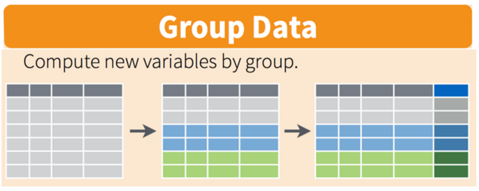
Figure 2: Visual depiction of the group_by() function.

Example: Median price by number of fireplaces

Let’s add a little nuance to the first question we asked about these data. Instead of asking “What is the typical price of a home?,” let’s ask: “does the typical home price depend on the number of fireplaces it has?”.

Looking through the SaratogaHouses data set and examining the fireplace variable, we see that there are 5 different groups of homes: homes with 0, 1, 2, 3 or 4 fireplaces in them. So to answer our question about these data, we take into account whether a home has 0, 1, 2, 3 or 4 fireplaces when computing the median price.

We can incorporate this information by grouping the data according to the fireplace variable and then summarizing the price variable.

Code

SaratogaHouses |>
  group_by(fireplaces) |>
  summarize(median_price = median(price))

# A tibble: 5 × 2
  fireplaces median_price
       <int>        <dbl>
1          0       158250
2          1       215700
3          2       277750
4          3       360500
5          4       700000

Since there were five different groups of homes (one group for each number of fireplaces), our resulting summary has 5 rows in it: one median price for each type of home. We can see that the price of a home strongly depends on the number of fireplaces it has: homes with more fireplaces have higher median prices.

Figure 3 provides a simple schematic for this calculation (based on a small subset of the data).

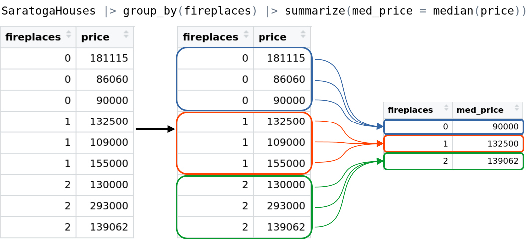
Figure 3: Grouping the SaratogaHouses data set by the fireplaces variable, then summarizing each group using the median price.

Now, it’s time for you to practice computing your own group-wise summaries.

Question

Does the price of a home depend on the type of heating system it has? To find out, use the incomplete code below as a template and compute the median price of all a homes, taking into the type of heating system the home has. Be sure to look back at the variables in the data set to figure out which one can tell you what type of heating system a home uses.

SaratogaHouses |>
  group_by(______) |>
  summarize(median_price = median(price))

Question

How does the average size of a home depend on the number of bedrooms in the home? Write your own code “from scratch” to compute this summary. Be sure to think about

1. Which variable should be the “grouping” variable (i.e., which variable you should look at to figure out which group a home belongs to) and
2. Which variable should be the summarized variable?

Example: Counting the number of homes without fireplaces

For almost all of R’s summary functions, you have to place the name of the variable you want to summarize inside the parentheses of the summary function you’ve chosen. For example, whenever we’ve computed the median price, we always wrote price inside the parentheses for the median() function.

However, there are exceptions to this rule among R’s most commonly-used summary functions. The most common is the n() function. The n() function counts the number of rows within each group of your data, which is very useful for summarizing categorical variables. In fact, knowing the number of observations in each group is so important that we recommend computing them every time you use the summarize() function, even when it may not be immediately obvious to you why that information is important.

Tip

Always compute the number of observations in each group with the n() function every time you use summarize().

For example, we could add the n() function to our previous example of computing the median home price grouped by the number of fireplaces, to learn exactly how many 0, 1, 2, 3 and 4 fireplaces homes exist in the data set. Since each row represents one home, counting the number of rows is the same as counting the number of homes!

Code

SaratogaHouses |>
  group_by(fireplaces) |>
  summarize(
    median_price = median(price),
    num_homes = n()
  )

# A tibble: 5 × 3
  fireplaces median_price num_homes
       <int>        <dbl>     <int>
1          0       158250       740
2          1       215700       942
3          2       277750        42
4          3       360500         2
5          4       700000         2

Not surprisingly, most homes have no fireplace, or just one fireplace. But we also learned that there were only two homes with three fireplaces, and only two more with four fireplaces. This is important because it tells us that the mean home prices are based on only two values (each), and are thus not robust. Furthermore, this example highlights how the syntax for using n() function is different from others: you don’t put anything inside the parentheses for the n() function!

This might seem confusing at first, but makes sense when you think about it for a moment. Since the n() function is just counting the number of rows, it doesn’t need to know anything about the contents of those rows. Your rows could have words, numbers, or pictures in them—but the n() function simply ignores all that, and counts how many rows there are. You don’t need to provide it any specific variables for it to do its job.

Question

Get some practice using the n() function to summarize the frequency of different category values by using the incomplete code below as a template to figure out how many homes use electric, gas, or oil as their heating fuel. Be sure to look back in the documentation for the SaratogaHouses data set to figure out which variable measures what kind of fuel a home uses, so you know which variable to group the data by!

SaratogaHouses |>
  group_by(____) |>
  summarize(num_homes = ____)

Question

Write your own code “from scratch” to calculate how many homes in the data set do and do not have a waterfront on their property.

Summarizing with Missing Values

When dealing with data, it’s usually the case that we don’t have values for every observation of every variable. It could be that the given variable doesn’t apply to the given observation, but usually, it’s just that the value is unknown for some reason. This unknown data is commonly referred to as missing data. Missing data in R is indicated by using NA in place of the data.

The SaratogaHouses dataset doesn’t have any missing data, but the penguins dataset in the palmerpenguins package does. Load that package using the library() function.

Let’s take a look at the average body mass in grams for each species of penguin:

Code

library(palmerpenguins)
penguins |>
  group_by(species) |>
  summarize(avg_body_mass_g = mean(body_mass_g))

# A tibble: 3 × 2
  species   avg_body_mass_g
  <fct>               <dbl>
1 Adelie                NA 
2 Chinstrap           3733.
3 Gentoo                NA 

With what we’ve learned so far, we can only see the average mass for chinstrap penguins while the average masses for Adelie and gentoo penguins are both NA. By default, the mean() function (and other similar functions) output NA if there are any NA values in the data. That’s because it’s important to note that with the information we have, we can’t take the average of all the observations.

When you see NA values in your data, it’s important to understand more about why they might appear. If we were looking at a variable measuring the length of each penguin’s chinstrap, we would expect to only see that value for chinstrap penguins and therefore get the above results. However, mass is something that all penguins have, so we would expect to be able to calculate an average for any species.

We also want to look at where and how often these NA values appear. One way to do this is filtering your dataset to show only observations where a certain variable is NA. We can do that by using the is.na() function within the filter() function. The below code shows an example of this being used to show only penguins with missing bill_length_mm.

Code

penguins |>
  filter(is.na(bill_length_mm))

Question

Use the is.na function and the penguins dataset to see only penguins with missing body mass.

You should see that there are only 2 penguins missing body mass observations, one Adelie and one gentoo, compared to 1728 total penguins. With so few missing values, it’s unlikely that the mean mass would change much even if the masses of these two penguins were serious outliers. In this type of case, it’s often okay to exclude the NA values and take the average of all known observations. If a large portion of the data (either overall or within a group) were missing, we might not want to do this.

We tell R to exclude NA values by using the na.rm argument of the mean() function. This argument removes NA values before the calculation. It’s an optional argument, meaning you don’t need to include it unless you want the default behavior of the function to change.

Question

Use the na.rm argument of the mean() function to calculate the average body mass in grams for each species of penguin with NA values removed. If you’re not sure how to add this argument, refer to the documentation for the mean() function.

You should now see numeric values for all three penguin species.

Many other functions that you use within summarize() will behave similarly to the mean() function here and will also have the na.rm optional argument.

Finishing this lab

Step 1: Create twin document

Download the Lab 5 template (if you haven’t done so already). Complete it such that the results in the generated output match the examples in the Lab 5 solutions file.

Step 2: Final Project Data Check 2

As part of your preparation from the final project, you need to identify data sources. In labs four through six, you will investigate a new data repository. Each week, you will identify one dataset that you are interested in. For each dataset, write one sentence explaining why you think this dataset could be a good fit for the project (save this for later). The data need to be downloadable (i.e., not from a package such as openintro or moderndive), and cannot be any data we have used in class. The data must also fit the following characteristics:

• Have at least 200 observations, and no more than 10000
• Have at least 4 variables total (not including ID variable)
  • At least 2 categorical variables
  • At least 2 numeric variables

Submit the name and URL for the data as part of each week’s Moodle quiz.

You are welcome to use data from any source that meets the above requirements. Here are a few resources to get you started:

• FiveThirtyEight makes the data they use in their articles publicly available.
• The UCI Machine Learning Repository has a collection of datasets used in machine learning.
• Kaggle has a large collection of user-uploaded datasets, often used in competitions hosted on the website.

Step 3: Complete the Moodle Quiz

After completing the data check, complete the Moodle quiz for this lab.

Footnotes

1. The summary function n() only works within a call to summarize(). The function length() computes the number of entries in any vector.

2. This is not a single function, but a construction that works most of the time (depending on what you are doing).