Lab 8: Formatting in Quarto

Why are we here?

A critical (and often neglected) aspect of conducting research is clearly communicating your work to a wider audience and making it easily digestible. The average person will not understand (or likely care about seeing) your code, and only needs to see the output. Additionally, the thoughtful use of formatting elements such as section headings, mathematical expressions, links, and images help to make your report more easily understood. At the end of the day, we want our rendered documents to look visually appealing so people want to read and understand them. Thankfully, we can accomplish all of this within Quarto, and we can render our reports into many different formats, such as HTML or PDF documents, slideshow presentations, or even entire websites!

Lab Goals

The first goal for this lab is to learn the basics of formatting Quarto documents. This includes general Markdown concepts like creating sections, links, text styling, lists, images, and footnotes. Additionally, you will learn the basics of how to control the rendered output by specifying global options via YAML and local options in specific chunks. After completing this lab, you should be able to use formatting to make your documents more professional and easier to read.

The second goal for this lab is to make substantial progress towards completing Phase 2 of the final project. For this phase, you will write an introduction to the data set you selected in Phase 1 that acquaints a reader with its topic, basic features, and its context.

In order to accomplish both goals at the same time, you’ll incorporate Quarto formatting skills into your work on Phase 2 of the project. You will know that you are done when have created a Quarto document that:

Provides scaffolding for all aspects of Phase 2
Includes the following stylistic elements:
- Section headers
- Italicized text
- Bolded text
- Text stylized as code
- At least one hyperlink
- At least one image
- At least one footnote
- At least one new global option in the YAML header
- At least one chunk option

Optional Reading

Quarto’s official documentation of it’s Markdown support is a great page to bookmark for future reference, and to learn about more advanced formatting features not covered in this lab.

The R Markdown Cheat Sheet is another great resource that demonstrates a variety of ways you can customize your document.

Lab instructions

Create your Quarto Document

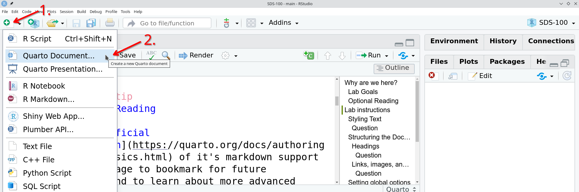
There is no Quarto template for this week’s lab. Instead, begin by clicking on the “New File” icon in the top-left corner of the RStudio window. Choose “Quarto document” from the drop-down menu that appears.

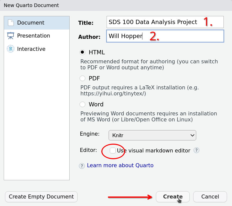
In the pop-up window, fill in the title and author. The title should be “SDS 100 Data Analysis Project”, and the author should be your name. Make sure that the “Use visual markdown editor” box is unchecked, and then press “Create”.

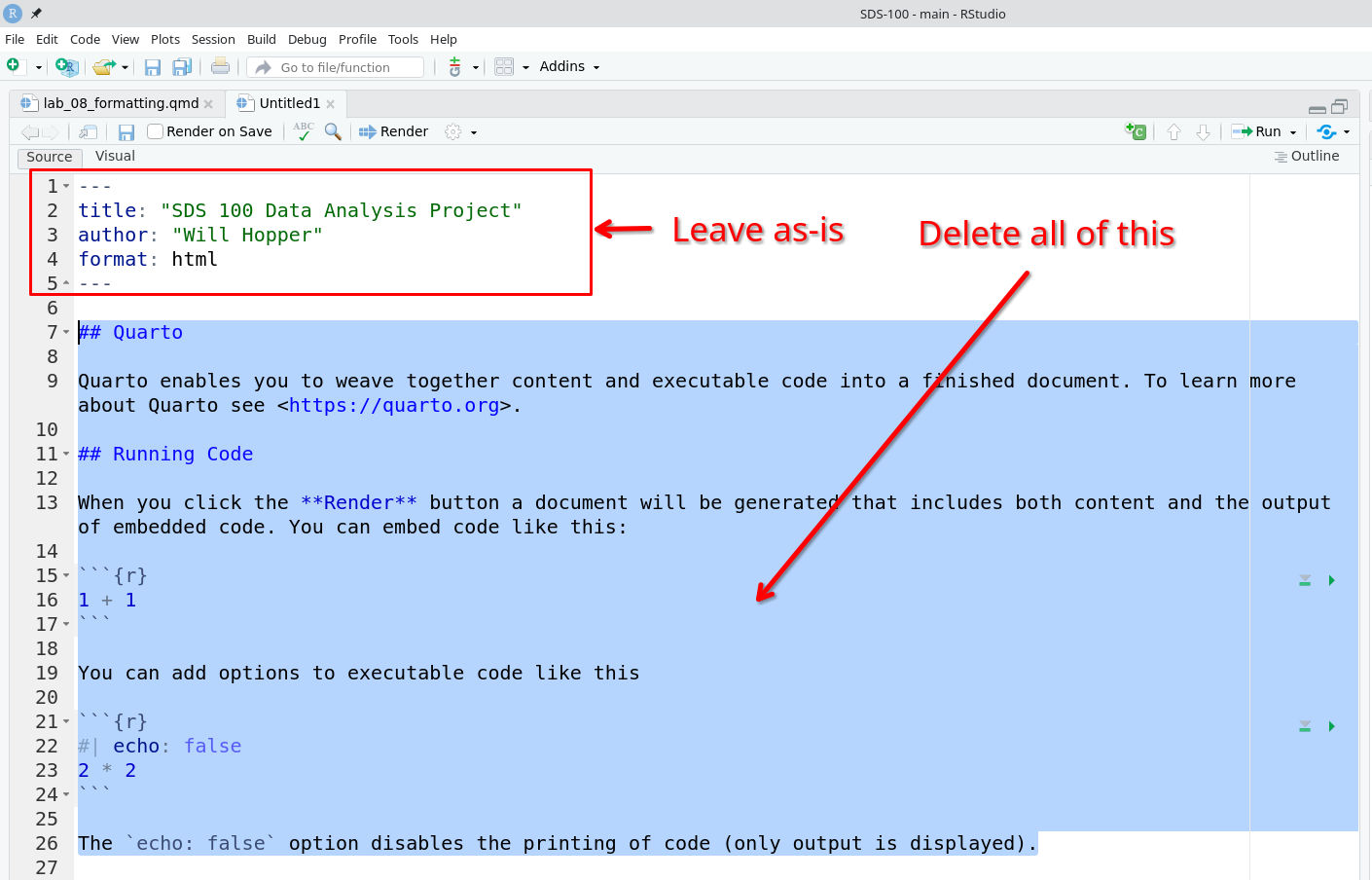
After clicking the “Create” button, a new Quarto document should open in the RStudio Editor pane. You should delete all the “boilerplate” text in this file, but leave the header at the top intact.

Finally, press the save button and save this Quarto document inside your SDS 100 project folder.

Review Phase 2 Requirements

Before beginning your work, take a few minutes to carefully read the expectations for Phase 2 of the project.

Headings

Sections heading are very helpful breaking up a long report into digestible chunks, and also forces you to organize your writing into clear, separate thoughts. A well-organized and labelled report also helps your reader quickly hunt down a specific piece of information they might be searching for.

You can generate section headings by placing a # character in front of the text that you want to become a section heading. You can create subheadings by adding additional # characters; each additional # makes the subheading go down another level. For example, ## creates a second level heading, and ### creates a third level header. Examples of each level are shown in Table 1:

Table 1: Markdown syntax for creating section headers

Markdown Syntax	Output
`# Header (Level 1)`	Header (Level 1)
`## Header (Level 2)`	Header (Level 2)
`### Header (Level 3)`	Header (Level 3)
`#### Header (Level 4)`	Header (Level 4)
`##### Header (Level 5)`	Header (Level 5)
`###### Header (Level 6)`	Header (Level 6)

Important

Be sure to leave a space between the # symbol and the start of the text in your header! Without this space, the header won’t appear correctly in your output.

For example # My Header will work, but #My Header won’t display correctly.

Question

Add level 1 headings for each of the following project phases to the Quarto document you just created:

Phase 2: Data Description
Phase 3: Summarization
Phase 4: Data Visualization
Phase 5: Ethics & Impact

Additionally, add the following level 2 headings underneath the Phase 2 heading:

Topic & Origin
Data Wrangling
Description of Variables

Then, render your Quarto document to be sure that your markdown formatting produces the expected output in your HTML document.

Styling Text

There are many ways to stylize your text. Note that these stylizing options only apply to text outside of chunks. Below are some of the most common stylizing features:

Putting a single * around a word or words will italicize text.
- For example, typing *R for Data Science* will italicize the text to look like R for Data Science
Similarly, a double ** around a word or words will bold the text.
- For example, typing **Hello World** will bold the text to look like Hello World
A single ` around a word or words will make the text styled as code.
- For example, typing `library(tidyverse)` will style the text in a monospaced font to look like library(tidyverse)

Please see Quarto’s official documentation for more even more examples of text styling possibilities.

Question

Reproduce the following sentences, including the formatting:

In the “Topic & Origin” section, write: The main research question my data can be used to address is: _________
In the “Data Wrangling” section, write: Data wrangling is the process of transforming “raw” data into the format you need for visualization and/or analysis.
In the “Description of Variables” section, write: The dplyr::glimpse() function can be used to get a quick overview of a data set’s contents.

Then, render your Quarto document to be sure that your markdown formatting produces the expected output in your HTML document.

HyperLinks

Links to URLs are a helpful tool to guide the reader to outside resources. An in-text hyperlink in markdown formatting has two components:

The text you want to appear in the document is placed inside square brackets
The URL you want to link to is placed inside parenthesis immediately after the square brackets

A few examples of a markdown formatted link, and the final result after rendering, are shown below:

Markdown Syntax	Output
`[Smith College](https://www.smith.edu)`	Smith College
`[Learn the Tidyverse](https://www.tidyverse.org/)`	Learn the Tidyverse

Question

In the “Topic and Origin”, write a sentence that begins “These data were retrieved from _________”, and replace the blank space with a link to a web page where the reader can download your data set.

Then, render your Quarto document to be sure that your markdown formatting produces the expected output in your HTML document.

Images

You can embed to an images in your rendered document with a very similar syntax. To embed an image, you:

Start with an exclamation point
Write the “alt text” (which is what screen readers use to describe the image for visually impaired people) for the image inside square brackets immediately after the exclamation point
- Depending on the context the image is rendered in, this “alt text” may also show up as a figure caption.
The path to the image file is placed inside parenthesis immediately after the square brackets
- The path to the image file could be a URL, or the path to a file on your computer

A few examples of a markdown formatted link, and the final result after rendering, are shown below:

Markdown Syntax	Output
`![dplyr logo](https://www.tidyverse.org/css/images/hex/dplyr.png)`
`![Quarto logo](gfx/quarto_logo.png)`

Question

Add an image in your “Topic & Origin” section that is related to the topic of your data set.

Then, render your Quarto document to be sure that your markdown formatting produces the expected output (an image) in your HTML document.

Footnotes

Footnotes are also a useful tool to provide the reader with more information/context that isn’t central to your text, but is easily accessible.

To write a footnote in markdown syntax:

Place a caret ^ in your text where you want the footnote reference to appear
Place square brackets immediately after the caret, and write the text of your footnote inside the square brackets

Some examples of footnotes in markdown formatting and the rendered output are shown below:

Markdown Syntax	Output
`Kingambit is a fair and balanced Pokemon^[He must be banned immediately].`	Kingambit is a fair and balanced Pokemon¹.
`There are two kinds of programming languages^[Languages people don't use use, and languages people complain about.].`	There are two kinds of programming languages²

Question

Include a footnote in the “Topic & Origin” section that includes information on the year(s) the data were collected. If the years are unknown, then indicate this in your footnote.

Then, render your Quarto document to be sure that your markdown formatting produces the expected output (a footnote) in your HTML document.

Setting global options

Every Quarto document starts with a block of settings written in a language called YAML. YAML headers are demarcated by three dashes (---) at the top and bottom. The configuration options in this section can be used to control what happens when the Quarto document is rendered into an output document.

For example, the YAML header for the Quarto document used to create this lab assignment looks like this:

---
title: "Lab 8: Formatting in Quarto"
editor: source
format: 
  html:
    code-fold: true
execute: 
  echo: true
knitr:
  opts_chunk: 
    message: false
---

Let’s walk through a few of these items.

title: Whatever you write here will appear in a large font at the top of the rendered document.
- Notice that the word title is followed immediately by a :, follow by a space, follow by the actual title text inside quotation marks.
- Unlike R code, where spacing is largely irrelevant, you must follow these precise spacing rules in the YAML header.
editor: The value source indicates this Quarto document should be viewed as a plain text
- We strongly recommend that you always use the source editor for all your Quarto documents.
- You should never use the visual editor; It looks pretty, but it frequently hides formatting mistakes that prevent your Quarto document from rendering.
format: The format option controls what type of output document is created when the Quarto document is rendered. This option can be very simple (e.g., format: html or format: pdf).

However, this YAML header specifies a more fine-grained configuration by beginning a nested list of setting. Note how the options here are successively nested by exactly two spaces of indentation. Whenever you need to use a nested list of settings, you must follow the “indent each level by two spaces” rule, or your Quarto document will not render.
- html: Having this nested beneath the format: option indicates that the output document should be an HTML document.
  - code-fold: true adds a button next to each code chunk in the HTML output that, when clicked, expands or contracts (i.e., shows or hides) that chunk of code.
execute: Options nested beneath execute: control the behavior of code chunks when the document is rendered.
- echo: true means that all code chunks will be displayed in the output document.
  
  There are many more code execution options that are useful on a regular basis. You can read about the full of execution options in the official Quarto documentation
knitr: these options are similar to those under execute, but the execute options apply to code chunks in any programming language Quarto can be used with (e.g., R, Python, SQL, ). Options in the knitr section apply only to R code chunks.
- chunk_opts: Options in this section apply to individual code chunks, instead of the entire document
  - message: false indicates that, if the R code produces any messages while it is running, those messages should not be included in the output document.

Embedding resources

One additional option that is important to add to your own Quarto documents is the embed-resources: true option. which belongs underneath the html: section of the header. You may remember this option from Lab 3, where we discussed it’s importance for making sure all your plots are embedded into your HTML output.

If you omit this option, your HTML document will lose all of its formatting and figures when you send it to someone over email or upload it to Moodle. This means its very important to use embed-resources: true in the global YAML header for your project, since you will be sharing your work with the other members of your group and turning in your work on Moodle.

Question

Edit the header of your final project Quarto document to include the embed-resources: true option. Feel free to refer back to the end of Lab 3 to see an example of the precise formatting. Remember, all the little spacing and indentation details matter in the YAML header!

Then, render your Quarto document to be sure that your YAML formatting is correct; if your document won’t render, you need to adjust your YAML formatting.

Chunk specific options

If there’s one rule that’s always true, its this: there are exceptions to every rule. That’s why Quarto gives you the ability to include chunk options inside each code chunk. These chunk-specific options allow you to override “global” options from the execute: and knitr: sections of the YAML header, and customize the behavior of each individual code chunk to your needs.

Here are some of the most commonly use chunk options

#| eval: true: Whether to evaluate (i.e., run) a code chunk. The value true indicates “Yes, run this code”, while a value of false indicates “No, don’t run this code”.
#| include: true: Whether to include anything from a code chunk in the rendered document. If include: false, the code will still be evaluated but the neither the code nor the output will be displayed.
#| echo: true: Whether to make the code visible in the rendered document. If set to false then only the output (but not the code) will be shown.
#| message: true: Whether to show any messages that appear when running a chunk.
#| warning: true: Whether to show any warnings that appear when running a chunk.
#| results: hide: Whether to hide the output from R.

Chunk options must be written at the very beginning of an code chunk to take effect. Also, take note of the special comment character #|, followed by a space, at the start of each chunk option. You must use this precise formatting for your chunk options, or the Quarto document will not render.

Here’s an example of a code chunk that uses the eval, echo, and message options to customize how the chunk is executed. The code in this chunk will be evaluated (i.e., it will be run), but the code will not be shown in the output document, and any warnings that occur will also not be shown in the output document.


```{r}
#| eval: true
#| echo: false
#| message: false
sample_def <- read_csv("data.csv")
```

Question

Insert a new code chunk in your Quarto document’s “Data Wrangling” section. In this code chunk, write code that will import your project data into R, and store it as an object in your environment.

If your data is stored in a CSV file, you can load the tidyverse package and use the read_csv() function
If your data is stored in a XLSX (i.e., an Excel file), you can load the readxl package and use the read_xlsx() function. You may need to install this package, since none of the previous labs in SDS 100 have asked you to install it.

Use chunk options to make sure that the code is hidden in when the document is rendered, and the no warnings or messages are displayed when the document is rendered either.

Then, render your Quarto document to be sure that your code and chunk options are formatted correctly.

Lists

You can use markdown formatting to produce both bulleted and numbered lists.

To produce a bulleted list, simply start each new line with a - character, and leave a space between the - and the text for each list item.

To produce a numbered list, simply start each new line with a numeral and a period (e.g., 1., 2., etc.)and leave a space between each numeral and the text for each list item.

A few examples of markdown lists are shown below. Be sure to leave at least one blank line before the start of your list, and at least one blank line after the end of your list!

Markdown formatting

The secrets to success, in no
particular order, are:

- Perseverance
- Preparation
- A little bit of luck

My favorite Pokemon are:

1. Sylveon
2. Calyrex-Shadow
3. Krookodile

Output

The secrets to success, in no particular order, are:

Perseverance
Preparation
A little bit of luck

My favorite Pokemon are:

Sylveon
Calyrex-Shadow
Krookodile

Question

Write a bulleted list in the “Description of Variables” that describes each of the variables in your data set.

Remember that you only need between 4 and 10 variables in your data set. If your data set has more than 10 variables, be sure to use the dplyr::select() function in the “Data Wrangling” section to choose at most 10 variables.

Next Steps

Step 1: Compare solutions

Double check that your Quarto document has all the necessary content and formatting elements by comparing your solutions against our example solutions. Each person will have a different topic, data set, and research question, so your answers won’t match word for word, but should have the same overall structure as the example solutions.

Be sure to render your Quarto document as well, to ensure that all your markdown formatting produces the expected output.

Step 2: Complete the Moodle Quiz

Complete the Moodle quiz for this lab.

Step 3: Complete the required reading

In preparation for next week’s discussion on Data Ethics and Algorithmic Bias, please engage with the following:

Step 4: Complete Phase 2 of the final project

Over the next two weeks, you will complete Phase 2 of the project, which is dedicating to providing contextually rich overview of your data sets’ contents. See the project page for complete details about what is expected during this phase of the project.

It’s important that you complete this phase with care and attention to detail, because your group members will be building on what you do in Phase 2 when they do their work in Phase 3.

References

Lum, Kristian, and William Isaac. 2016. “To Predict and Serve?” Significance 13 (5): 14–19.

Footnotes

He must be banned immediately↩︎
Languages people don’t use use, and languages people complain about.↩︎

Why are we here?

Lab instructions

Create your Quarto Document

Review Phase 2 Requirements

Headings

Header (Level 1)

Header (Level 2)

Header (Level 3)

Header (Level 4)

Header (Level 5)

Header (Level 6)

Question

Styling Text

Question

HyperLinks

Question

Images

Question

Footnotes

Question

Setting global options

Embedding resources

Question

Chunk specific options

Question

Lists

Markdown formatting

Output

Question

Next Steps

Step 1: Compare solutions

Step 2: Complete the Moodle Quiz

Step 3: Complete the required reading

Step 4: Complete Phase 2 of the final project

References

Footnotes